CDK2 Clustering

1. The simplest way to cluster structures based upon residue properties is to use the polyphony_Ete2_tree.py script. This will generate an interactive tree in Ete and write out a Newick format file. This is a standard tree text format and can be read in using a number of programs. Here is a dendrogram produced using FigTree. It shows the CDK2 chains clustered by Tanimoto similarity of the residue interaction fingerprints generated from protein-protein interaction database Piccolo (-p ppi option).

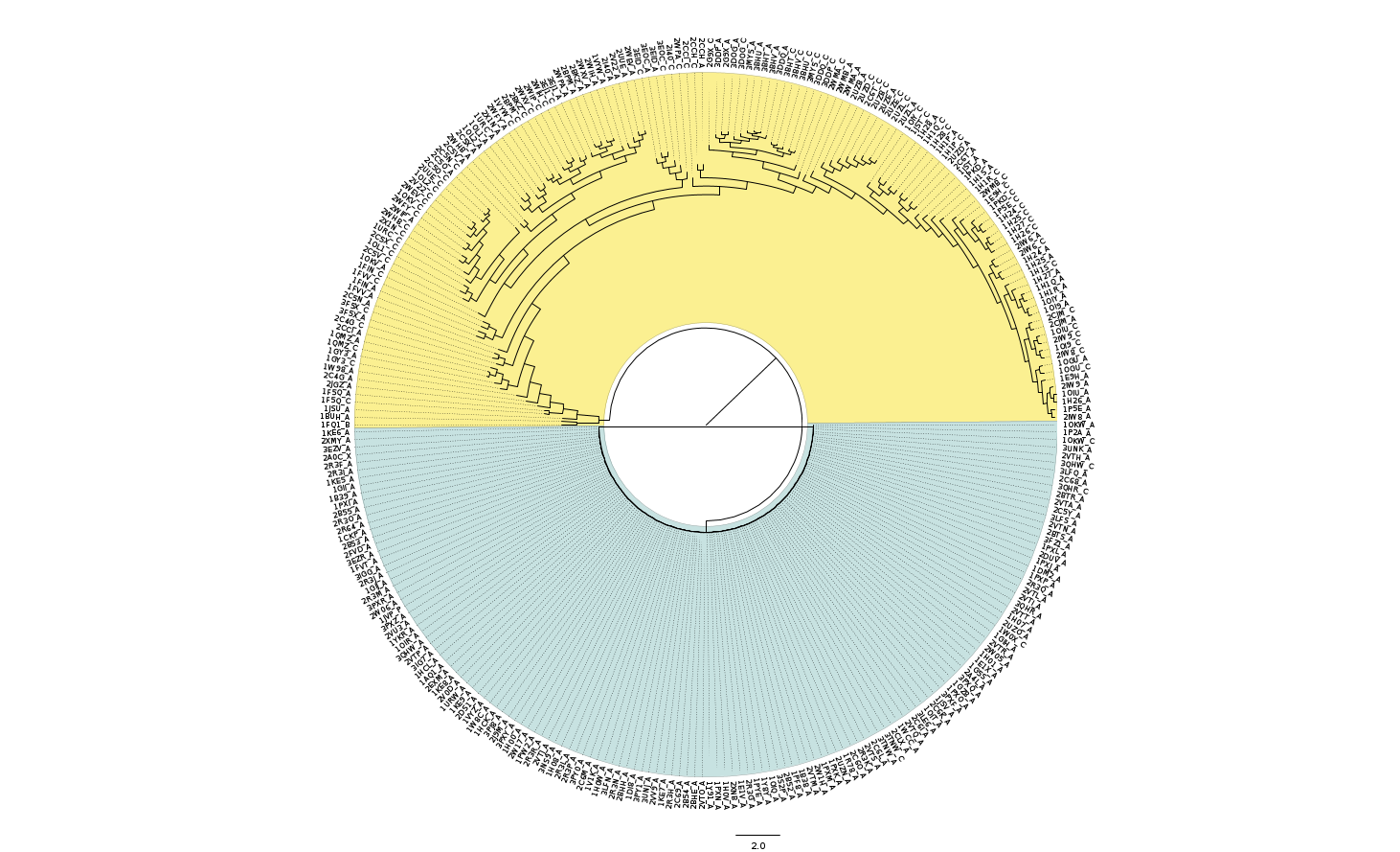
It shows the chains with no biologically relivant protein contacts in blue and those interacting, usually with cyclin a, in yellow.

2. Groups can be generated from the hierarchical clustering. This isn’t done in a very sophisticated way. One way is to use:

This method works well to split CDK2 chains into monomers and multimers (blue and yellow in above diagram).

e.g.

from Polyphony.Trees import Tree
from Polyphony.Comparison_Matrices import Structure_Matrix
from Polyphony.Structural_Alignment import Structural_Alignment
from Polyphony.Utils import Properties
from Polyphony.Plotting import plot_alignment_properties

## Main program

# Alignment file etc.
filename = "clust_1HCK_A_95.fasta"
update = False
property = "backbone"

# Create structural alignment
aligned = Structural_Alignment()
aligned.add_alignment(filename)

# Get/calculate selected property
properties = Properties()
array = properties.get_array(property, aligned, update)

# Cluster by protein-protein interactions
clust_array = properties.get_array("ppi", aligned, update)
structmat = Structure_Matrix(clust_array)
tree = Tree(structmat.data, structmat.get_labels())

# Group into active and inactive
groups = tree.biggest_left_right_others(1)
unbound = groups[0]
bound = groups[1]

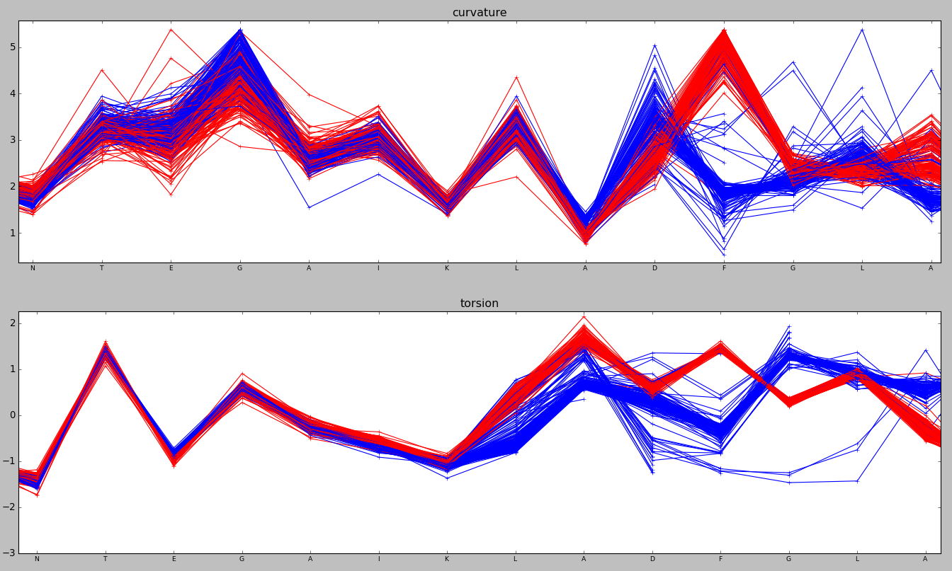
# Plot curvature and torsion, coloured by group
xlabels = aligned.get_consensus_sequence()
plot_alignment_properties(array.data, property, xlabels, array.dim_names, colour_groups=[unbound, bound])

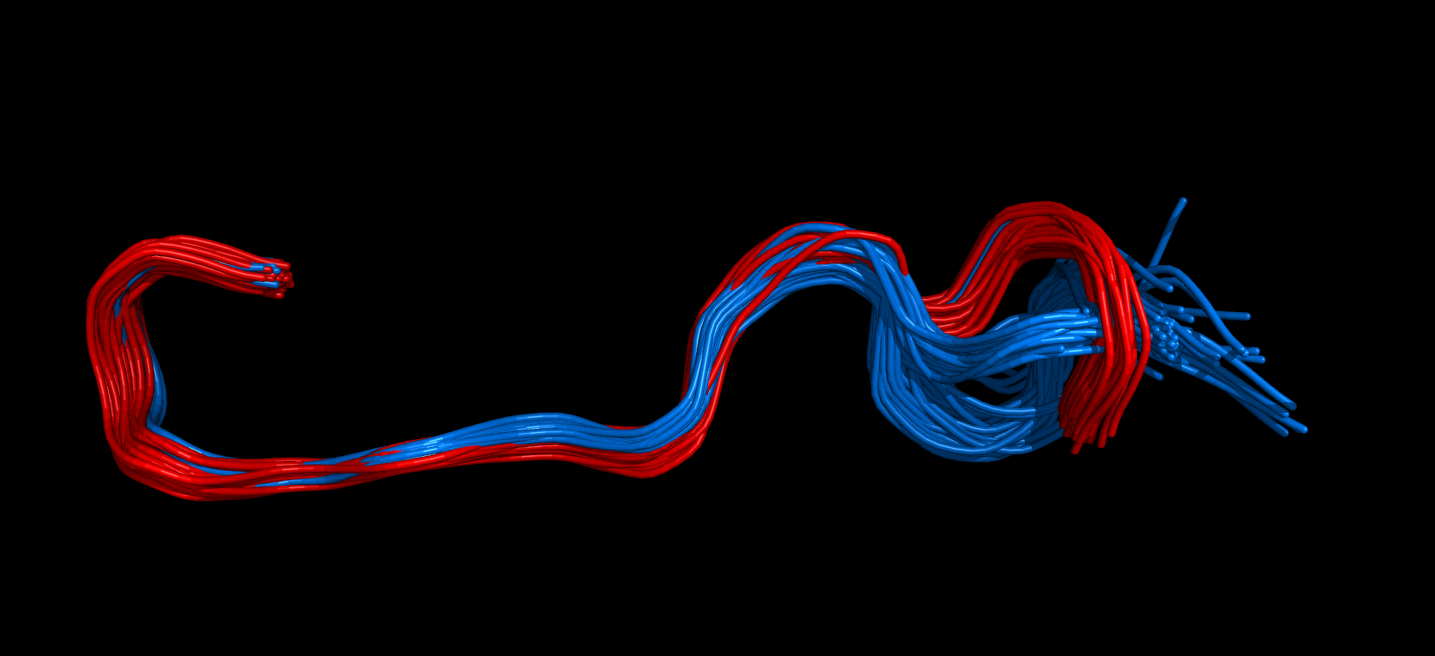
The same region can be visualised in 3D using in PyMol. Type pymol -R in one console window and run the following in another, preferably in ipython.

from Polyphony.Pymol import Pymol_Viz

# Get started and load representative structure into PyMol
cdk2 = Pymol_Viz("clust_1HCK_A_95.fasta","cdk2")

# Group in to bound and unbound structures
groups = cdk2.group_biggest_clusters(property="ppi")
unbound = groups[0]
bound = groups[1]

# Convert the lists of alignment index numbers to chain ids
unbound_ids = cdk2.ids_for_groups(unbound)
bound_ids = cdk2.ids_for_groups(bound)

# Find preferred segment of structurally conserved residues. Try experimenting with the cutoff. The default value of 0.5 can be a bit high.
cdk2.colour_conserved_segments(0.1)

# Load all structures in each group into a PyMol group allowing them to be coloured separately
# They then aligned using your chosen segment. This will take a few minutes
cdk2.load_structures(id_list=unbound_ids, segment=[101,111], pymol_group="unbound")
cdk2.load_structures(id_list=bound_ids, segment=[101,111], pymol_group="bound")

You can then colour each group separately, view as ribbons etc.