3. Using the PyMOL interface

You will obviously need to have pymol installed before you can do this. See Optional Add-ons for more information.

You are now ready to visualise in Pymol. To do this:

1. in a shell

pymol -R

don’t open more than one instance of pymol in this way at the same time, things get a bit confused.

2. in another shell, cd to the directory containing your fasta file
3. start ipython (interactive python, see Dependencies)

ipython

4. you can now show properties of your alignment mapped on to the structure loaded in pymol using python commands typed in your ipython session
5. firstly import the Polyphony package, then create a Pymol_Viz object for your alignment e.g.

from Polyphony.Pymol import Pymol_Viz
il2_viz = Pymol_Viz("clust_1PW6_A_95.fasta","il2")

the second argument is your choice of the name of the pymol group to be used to collect together visualisations of from the fasta file named in the 1st argument. This will create a group in pymol and load the representative structure. This is chosen automatically but you can override this choice by using the optional parameter e.g. chain_id=”1PW6_A”

6. use the tab completion feature of ipython to see what functions are available e.g. il2_viz.<tab>

7. use a question mark to see any documentation available e.g. il2_viz.colour_by_variability?

8. try one of the functions e.g.

il2_viz.colour_by_variability()

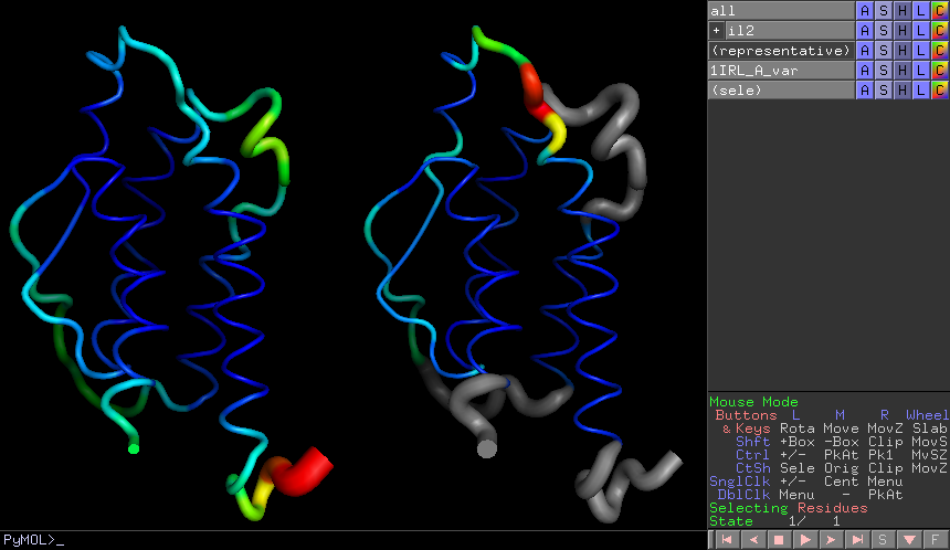
Please note that the first time you run these commands it may take some time to run, especially if you have many and/or very long sequences. Subsequent runs will be very quick because the results of time consuming calculations are stored for later use. Here’s what it should look like:

The thicker and redder the tube the more the structures vary between each other. Grey tubes indicate regions that are usually disordered.

9. copy your chain to another object in pymol (not in the ipython window) e.g.

copy 1IRL_A_var, 1IRL_A

to see multiple visualisations on the same structure. Please note, the name of the copy should start with the name of the original.

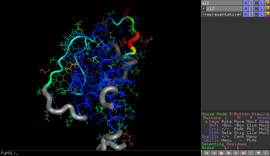
10. You can now display other properties and compare the results side by side using pymol’s grid by object display option e.g.

il2_viz.colour_by_average_bfactor()

In this case the very high average bfactor of n-terminus meant that it was red while the rest of the structure was blue. You can adjust the using the spectrum command in pymol. Values are stored in the place of the normal b-factors. E.g.

spectrum b, rainbow, 1IRL_A, 0, 20